📍 Walkthrough: particle-tracking microrheology
Track 400 nm tracers diffusing in water, build the mean-squared displacement, and read off viscosity and viscoelastic moduli — the classic Crocker–Grier workflow (doi:10.1006/jcis.1996.0217).
🖥️ Desktop / Colab only — this path needs
trackpy, which ships no wheels and can’t install in Pyodide. For the browser-friendly path see the DDM walkthrough.
1. The idea
A micron-sized tracer in a fluid jiggles by Brownian motion. In water the motion is purely diffusive: ⟨Δr²(τ)⟩ = 4Dτ (2D tracking), and Stokes–Einstein connects the diffusion coefficient to viscosity, η = kT/(6πηaD)… more precisely η = kT/(6πaD). In a viscoelastic fluid the MSD bends — and the generalized Stokes–Einstein relation turns the whole MSD curve into G′(ω), G″(ω).
2. Load the video
The low-concentration water video — sparse enough that individual tracers can be followed:
import microrheology as mr

path = mr.data.water_video("low")          # downloads once, caches
video = mr.read_video(path, fps=100, muperpix=0.1)
print(video)                               # n_frames, shape, fps, µm/px
3. Locate particles
trackpy.locate finds bright spots frame by frame (Crocker–Grier):
features = mr.tracking.batch_locate(video, diameter=15,
                                    minmass=1000, invert=True)
features.head()
diameter ≈ particle size in pixels; minmass rejects noise.
invert=True for dark particles on bright background.
4. Link into trajectories
traj = mr.tracking.link_trajectories(features, search_range=5,
                                     memory=3, min_length=50)
search_range (px) is how far a particle may jump between frames;
memory bridges brief disappearances; stubs shorter than
min_length frames are dropped.
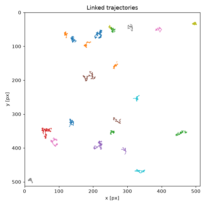
On the bundled water video this finds 4,545 features and links them into 23 trajectories of ≥ 50 frames:
5. Mean-squared displacement
msd = mr.tracking.mean_squared_displacement(traj, muperpix=0.1, fps=100)

import matplotlib.pyplot as plt
plt.loglog(msd.index, msd.values, "o")
plt.xlabel("lag time τ [s]"); plt.ylabel("MSD [µm²]")
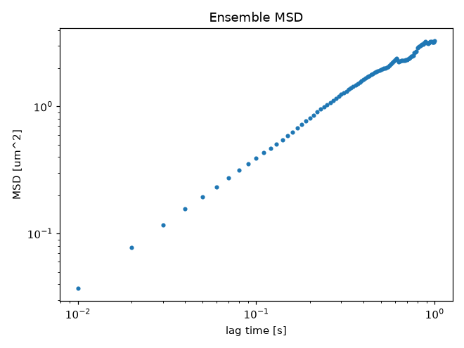
For water the log–log slope is 1 (diffusive). On the bundled video the ensemble MSD comes out straight with slope ≈ 0.96:
6. Viscosity from the MSD
out = mr.tracking.viscosity_from_msd(msd.index, msd.values,
                                     temperature_C=25.0, radius_um=0.2)
print(out)
# {'eta_Pa_s': ~1e-3, 'D_um2_s': ..., 'loglog_slope': ~1.0}
Water at 25 °C is 0.89 mPa·s — the fitted value should land nearby.
On the bundled video the fit returns η ≈ 1.2 mPa·s (D ≈ 0.90 µm²/s, log–log slope ≈ 0.96) — close to the literature value, from a 3-second compressed clip.
7. Moduli from the MSD (GSER)
omega, Gstar = mr.gser.msd_to_moduli(msd.index, msd.values,
                                     radius_um=0.2, temperature_K=298.15)

plt.loglog(omega, Gstar.real, label="G′")
plt.loglog(omega, Gstar.imag, label="G″")
plt.xlabel("ω [rad/s]"); plt.ylabel("modulus [Pa]"); plt.legend()
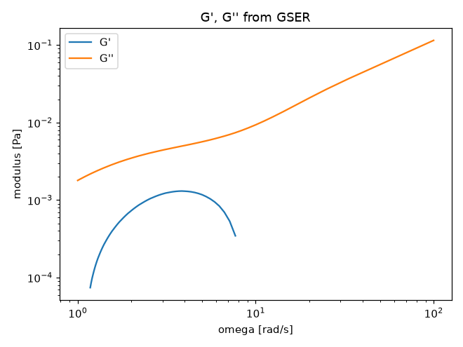
For a Newtonian fluid G″ dominates and grows ∝ ω while G′ ≈ 0 — the GSER of a straight diffusive MSD. In a complex fluid the curves cross and bend, and that is the fingerprint.
The bundled water video gives exactly that picture — G″ dominant and growing with ω, G′ small and noise-limited (a 3-second clip only goes so far):