🌊 Walkthrough: differential dynamic microscopy (DDM)
Measure diffusion — and hence viscosity — from a microscopy movie without tracking a single particle. DDM works even when tracers are too dense to resolve individually.
💻 Browser-friendly — this path needs only numpy/scipy/pandas, OpenCV for reading, and lmfit for fitting. It runs in JupyterLite/Pyodide.
Reference: Cerbino, R. & Trappe, V., Phys. Rev. Lett. 100, 188102 (2008). doi:10.1103/PhysRevLett.100.188102
1. The idea
Take two frames separated by a lag Δt and subtract them: static background cancels, and only what moved survives. Fourier-transform the difference and azimuthally average → the image structure function D(q, Δt). For Brownian particles it relaxes as a single exponential,
so each wavevector q gives a relaxation time τ(q) = 1/(Dq²), and a power-law fit over q yields D. Stokes–Einstein does the rest.
2. Load the video
The high-concentration water video — too dense for tracking, perfect for DDM:
import microrheology as mr

path = mr.data.water_video("high")
video = mr.read_video(path, fps=100, muperpix=0.1)
3. Explore the signal
Before the heavy computation, look at a frame pair, its difference, and the FFT power spectrum:
mr.ddm.browse_ddm(video) # interactive widget
You should see the difference image light up with motion and the power spectrum peak at low q.
4. Compute D(q, Δt)
D = mr.ddm.calculate_ddm(video, n_average=20, n_deltas=10,
                          interval=0.01, muperpix=0.1)
D.shape   # (n_deltas, n_q)
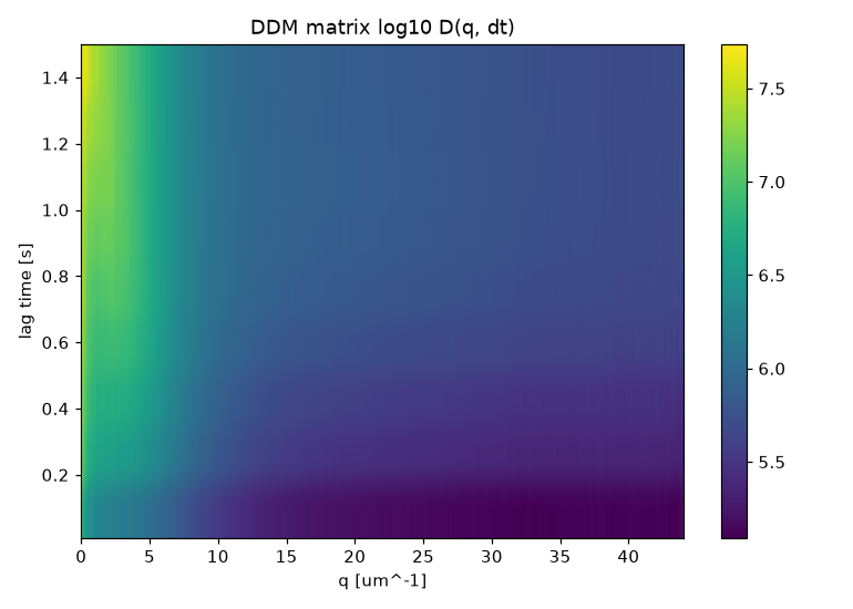
n_average frame pairs are averaged per lag; n_deltas lag times
are log-spaced. This is the expensive step — a few minutes on a
laptop for the full video. What it produces, for the bundled water
video, is a relaxation that grows with lag time and dies off with
q:
Inspect a slice interactively, with per-q fits:
mr.ddm.explore_ddm(video)
5. Viscosity
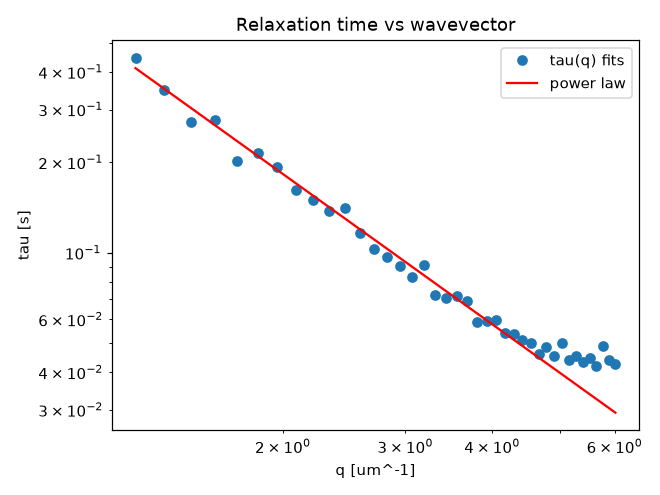
Each q-slice is fit to the single-exponential model; τ(q) ∝ 1/q² gives D, and Stokes–Einstein gives η:
eta = mr.ddm.viscosity_from_ddm(video, radius_um=0.2,
                                qmin=10, qmax=50, plot=True)
print(f"η = {eta:.3e} Pa·s")   # water ≈ 0.89e-3
(qmin/qmax select the clean mid-q range, away from the
low-q drift and high-q noise.)
On the bundled water video this gives η ≈ 0.63 mPa·s — the right order of magnitude for water at 25 °C (0.89 mPa·s), from a heavily compressed mp4 and no particle tracking at all. The per-q relaxation times follow τ ∝ 1/q² cleanly:
6. Or the radius
If the viscosity is known instead, the same pipeline returns the tracer size:
a = mr.ddm.radius_from_ddm(video, viscosity=0.89e-3,
                           qmin=10, qmax=50)
print(f"a = {a:.3f} µm")   # nominal 0.2 µm radius
On the bundled video this returns a ≈ 0.142 µm, vs the nominal 0.2 µm tracer radius — again in the right ballpark for a compressed demo clip.